1. Task - Exterior wall with interior insulation
In this tutorial, a typical historic masonry wall will be analyzed, created and simulated before and after applying interior insulation.
First, the existing construction (without interior insulation) is evaluated for thermal and hygric performance. Then, a variation study is performed to ultimately identify a suitable interior insulation system.
2. Part 1 - Simulation of the existing construction
This part of the tutorial deals with the basic steps to create a DELPHIN project.
2.1. Project creation with the project assistant
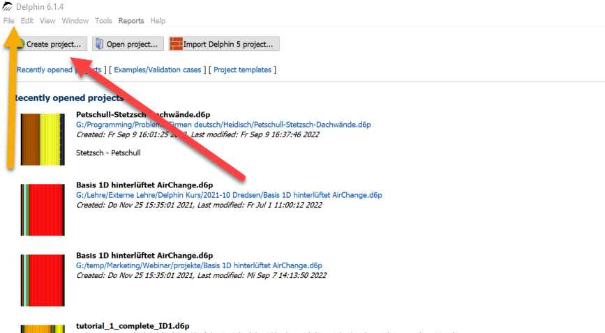
After starting DELPHIN, several buttons for creating and controlling a project are available in the upper left area of the main window. The first step is the creation of a new project. The button 'Create project' (or >> File >> New) opens a project assistant.
The project starts first with the info window shown below.
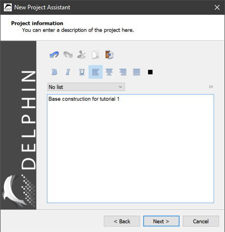
The wizard will guide you through the first steps. After confirming by clicking on 'Next' a dialog opens where project information can be entered (see next picture). The description will be displayed on the screen the next time DELPHIN is started.
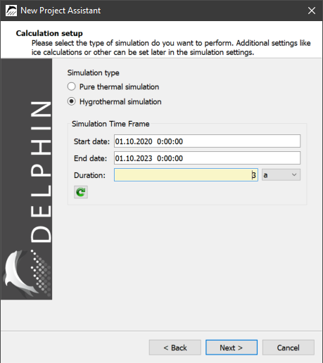
In the next window you can specify the calculation type as well as start and duration of the calculation. Mostly 'hygrothermal calculation' should be selected as calculation type. Purely thermal calculations are almost only useful for thermal bridge calculations. As start date the 1.1.2020 is preset. For normal climate data to be used cyclically, the year does not matter. For a measurement it can be useful to choose 1.10. as start date. This way, a full winter period is available right at the start. At least 3 years should be chosen as calculation period. If this should be too little for a measurement, the project can be changed and continued afterwards.
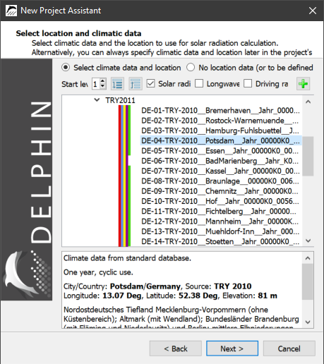
The next dialog is used to select the location. Here, you can choose from a list of locations for which hourly data are stored for DELPHIN. In this tutorial, the location TRY 2010 Potsdam, Germany should be used.
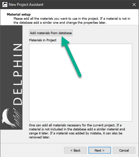
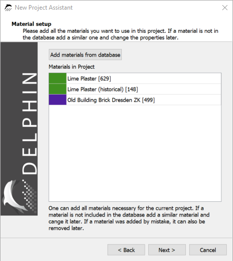
After that follows the material selection. To do this, click on the button 'Add materials from database' in the dialog shown below.
Then the material database selection opens.
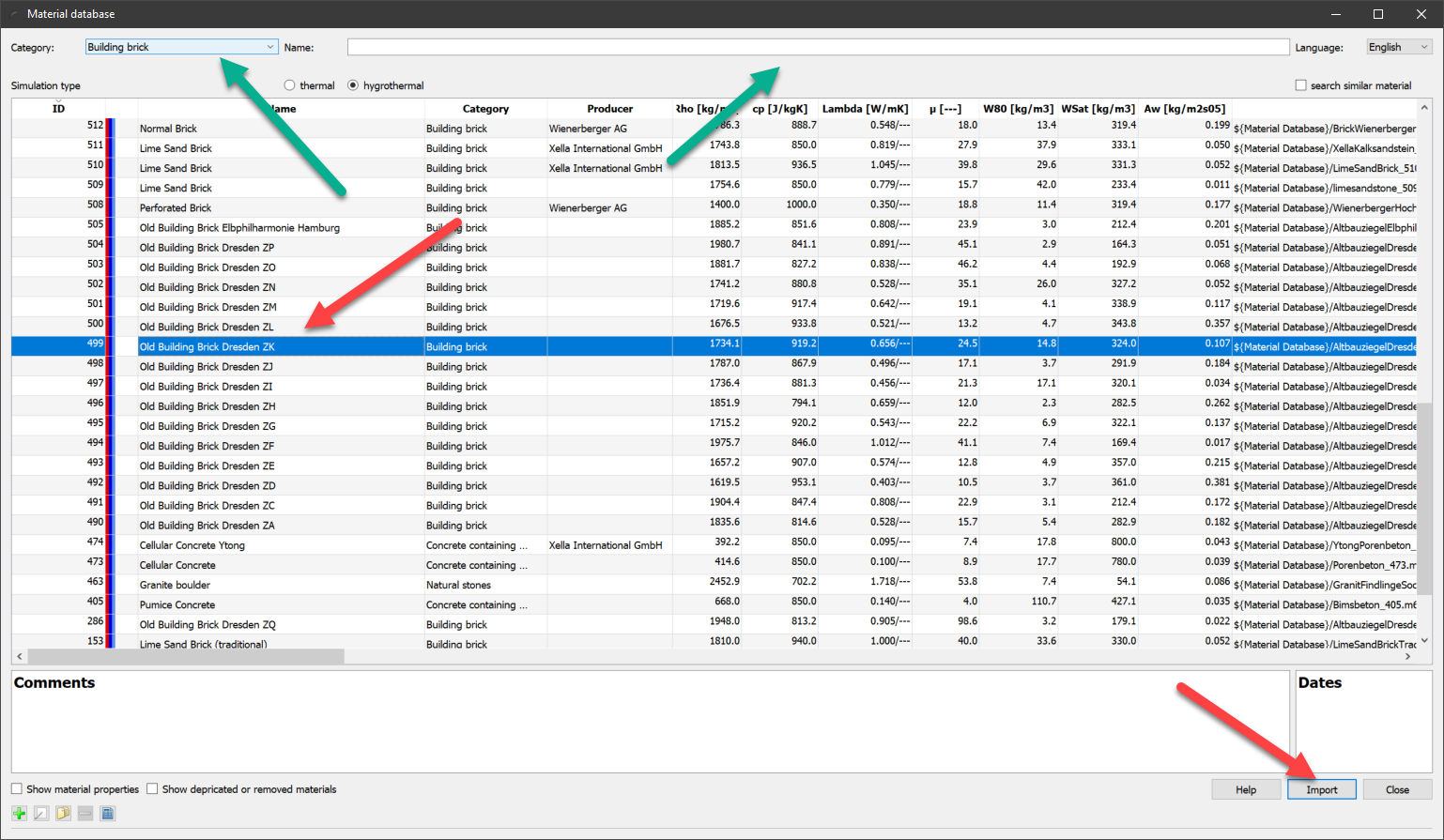
Here you can select materials and add them to the project by clicking the 'Import' button (red arrows). For the existing construction we need 3 materials:
-
Brick masonry (e.g. Old Building Brick ZK with the ID 499).
-
Interior plaster (e.g. lime Plaster (historical) ID 148)
-
Exterior plaster (e.g. lime Plaster ID 629)
The material database view shows the material name, manufacturer (if known) and some basic properties. Equally important is the material ID (first column). This is a unique ID that facilitates the identification of materials in each case. Next to it there is a color code which represents the transport properties. The colors have the following meaning:
-
Red - heat transport calculation possible
-
Dark blue - liquid water transport possible
-
Blue - vapor transport possible
-
Light blue - air transport possible
A single red bar therefore means that only heat transport processes but no moisture transport can be calculated for this material. For this example, characteristic values for hygrothermal calculations must be available for all materials. You can filter the display so that only such materials are shown. To do this, select 'hygrothermal' at the top of the dialog under 'Simulation type'.
Further there is a filter for material categories and a filter for the name (green arrows). For example, the masonry can be found faster if you select 'building brick' for the category. Clicking 'Import' adds the material to the project. Proceed in the same way for the two plasters. A detailed description of the material database dialog can be found https://www.bauklimatik-dresden.de/delphin/2nd/doc/D6_1_MaterialDBDialog/MaterialDBDialog_D6.1.2_en.html [here].
After the material selection has been closed, you return to the project wizard. Here you can see a list of the added materials.
The display colors of the materials can be changed later.
In the next dialog you can set the geometry.
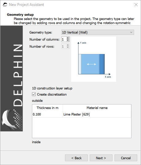
Here the basic geometry type can be selected, as well as the number of layers. Since a one-dimensional wall is to be calculated, '1D vertical (wall)' is the correct selection. The construction type can be changed later. The as-built construction consists of three layers (columns). For one-dimensional constructions, you can also set the layer thicknesses and assign the previously selected materials. The following figure shows the dialog after the following steps:
-
select as type '1D Vertical (Wall)'.
-
set number of layers to 3
-
enter layer thicknesses (outside is on top)
-
select materials
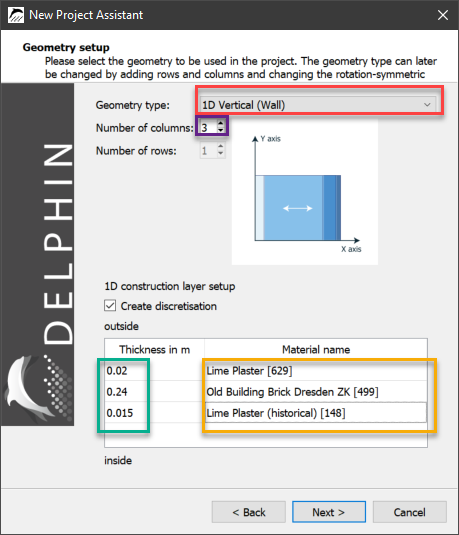
If 'Create Discretization' is checked, the layers are created in the project, the materials are assigned and finally everything is discretized. After clicking 'Next' the dialog for the surfaces (boundary conditions) appears.
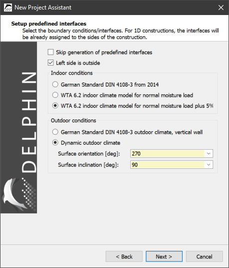
Checking the top selection will skip this dialog. The boundary conditions must then be defined manually. In the second selection box you can define where the outside should be. If this box is checked, left is outside, otherwise right. In this tutorial the left side should be outside, so the checkbox must keep unchanged. The assignment of the materials in the previous dialog will be adjusted if necessary. After that, the indoor climate and the outdoor climate are set. Here the following is selected:
-
For the interior climate, a climate calculated according to WTA leaflet 6.2 with a normal moisture load +5% is selected. This climate is also recommended as the design climate for living spaces according to DIN 4108-3.
-
For the outdoor climate, the data of the previously set climate location are taken. The inclination is 90°, i.e. a vertical wall. This wall is oriented to the west (270°). In Germany, this orientation is usually associated with the highest rain loads.
When you click on 'Next', the selected surfaces are generated and assigned to the construction. .Project wizard - outputs image::new_project_assistent_10_en.png[new_project_assistent_10_en,width=500,pdfwidth=10cm]
With the above settings, all fields ("colorful images") or profiles are output every 1.5 days. For the other outputs an hourly output rhythm is used. With the outputs selected here, even simple assessments can be carried out and the moisture behavior over time can be displayed. For example, the integral moisture mass indicates whether or not the construction will moisten in the long term, and the temperature and humidity on the inner surface can be used to estimate the risk for mold. More outputs can be added later. More information about the outputs can be found https://www.bauklimatik-dresden.de/delphin/2nd/doc/DELPHIN6_Outputs/Tutorial_4_D6_Outputs_en.html [here]. Since version 6.1.5, a settings dialog for assessments appears after clicking 'Next'.
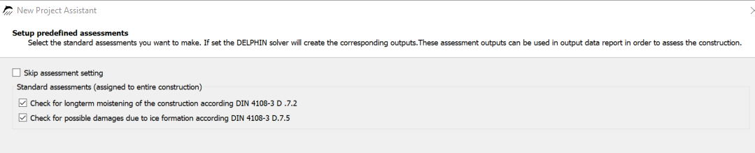
Here you can set whether DELPHIN automatically creates outputs for this project that are required for the following two assessments:
-
check for long-term moistening
-
Check for frost damage risk
The automatically created outputs do not appear in the output list. However, they are created and assigned to the construction. Since the names are defined, these outputs can then be used by the output and assessment report. The result of the assessment is then displayed there. With this dialog the project wizard ends. After clicking Close the main window is displayed.
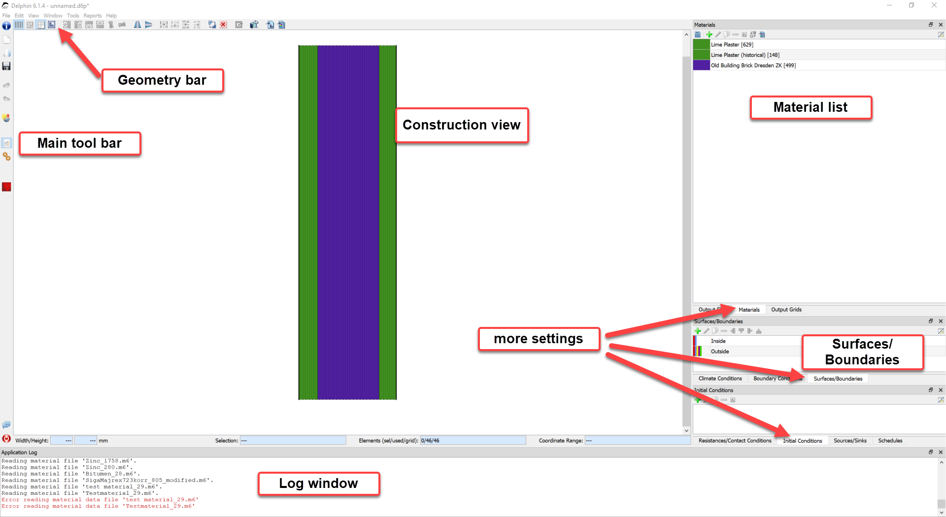
The image above shows the different areas of the main window. The layout of the different windows is very flexible. The different definition lists can be shown and hidden by using the window menu on the upper left bar. They can also be moved around and grouped into new tabs as desired. For this and following tutorials, the default layout will be left as is.
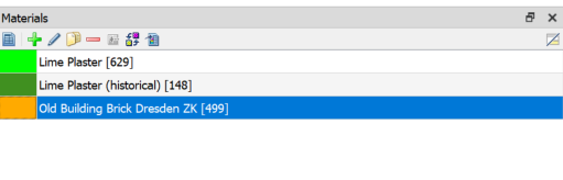
2.2. Customize material references
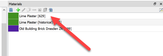
The project is basically ready for calculation. You can still edit the project now. Currently two materials use the same color (both plasters are green). This complicates the overview. To change this, first double-click on the top material (lime plaster).
This opens the assignment dialog for the material.
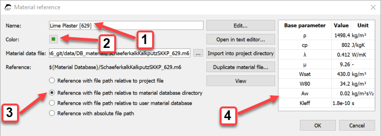
The name (1) serves in principle only as description and identification of the material and can be changed at any time. Likewise the color (2) serves only as differentiation in the construction window and can be changed just as simply by a click. Finally, the way in which the path to the material file is saved can be modified (3). This is especially important when project data is copied from one computer to another where the path structure is different. For this reason, it is usually recommended to use relative paths and to save project-related files, such as custom climates or material files, close to the project. On the right side of the dialog (4) a selection of material parameters is displayed. For this tutorial only the display color of the materials shall be adjusted. A click on the color opens a dialog for color selection. Different colors should be selected for all materials used. The color white (no assignment) should be avoided. The following figure shows the material list with changed colors for lime plaster and brick.
2.3. Surfaces and boundary conditions
The boundary conditions have already been created and assigned by the project wizard.
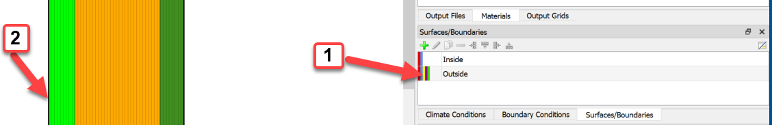
In DELPHIN 6, a distinction is made between interfaces and boundary conditions. A boundary condition describes a specific flow over an boundary of the structure (e.g. heat or vapor transport). A surface is a collection of boundary conditions with some additional information. In the lower right corner of DELPHIN (1) the list of existing surfaces is shown. Here there are surfaces for inside and outside. The colored markers indicate which boundary conditions are used:
-
Red - heat transfer
-
Blue - vapor diffusion
-
Yellow - short wave solar radiation
-
Brown - long-wave radiation balance
-
Green - driving rain
-
Dark blue - water contact
-
Light blue - air flow
If a surface is marked in the list (click), the assignment to the construction is shown as a thick dashed line in the view (2). A double click on a surface opens the settings dialog.
Only surfaces can be assigned to the construction. Boundary conditions can only be assigned to surfaces and climate conditions can only be assigned to boundary conditions. More about this later.
2.4. Outputs
Now a look at the outputs. In this tutorial the following outputs are used:
-
Temperature profile - time resolved temperature profiles through the whole construction.
-
Humidity profile - time resolved humidity profiles through the whole construction
-
Water content profile - time resolved water content profiles through the whole construction
-
Moisture content integral - moisture mass in the whole construction
-
Surface temperature inside surface - temperature on the room side surface
-
surface humidity inner surface - relative humidity on the room side surface
-
Surface temperature outside surface - temperature on the outside surface
-
Surface humidity outside surface - relative humidity on the outside surface
-
Surface heat flux inside surface - heat flux density on the room side surface
-
Surface heat flux outer surface - heat flux density on the outer surface
All outputs were defined and assigned by the 'Project Wizard'. As an example, an output for a saturation degree of the outer brick layer shall be added now. The degree of saturation can be used e.g. for the evaluation of the frost risk according to DIN 4108-3 D. To do this, proceed as follows:
Create output
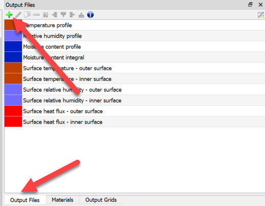
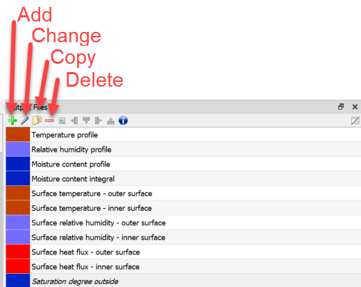
First select the tab for the output files. Then click on the green plus symbol in the upper left corner. This opens the output creation dialog.
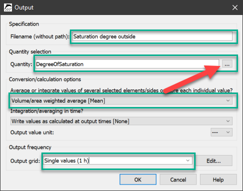
In the image above, all fields to be changed are outlined in green.
-
Input of a new name (it is also the file name)
-
Selection of the quantity to be output
-
Click on the selection button (red arrow)
-
Selection of the quantity in the dialog that then appears
-
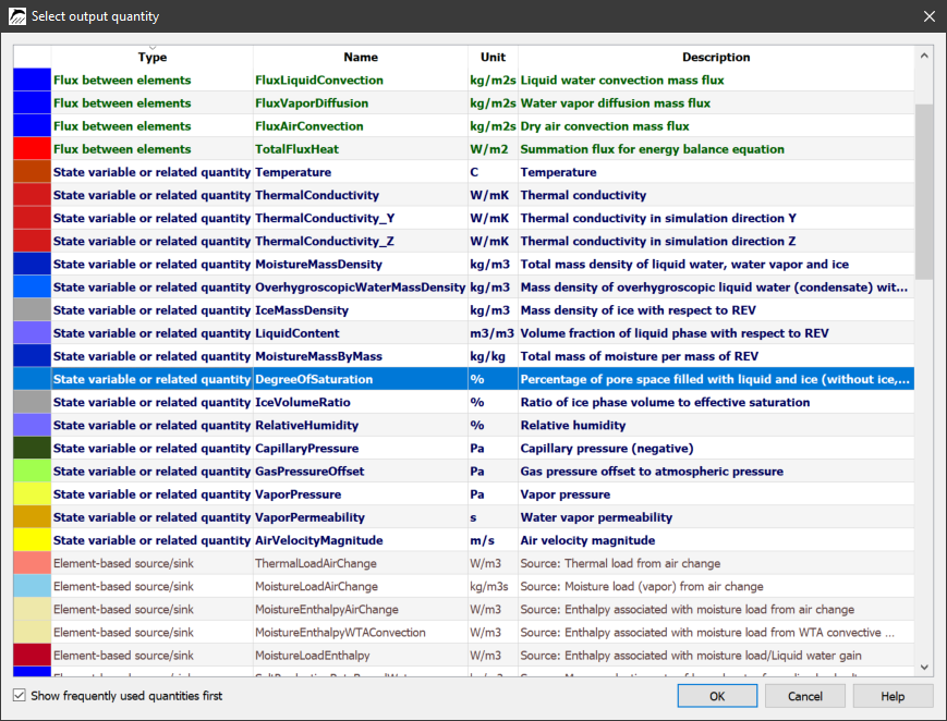
-
Set calculation option for space to 'volume/area weighted mean [Mean]'.
-
this will calculate a mean value over all selected elements
-
-
In the output grid select 'Single values (1 h)'.
When the settings have been adjusted as seen above, the dialog can be closed. The new output now appears in the output list.
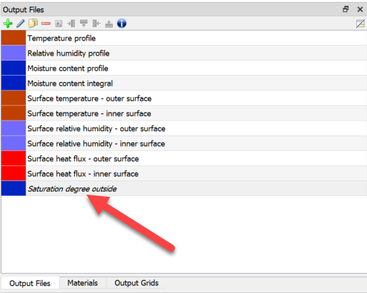
But the new output 'saturation' is shown in italics. This means the output is created but not yet assigned to the construction. This is to be done now.
-
Selection of the elements to which the output is to be assigned
-
here an approx. 1cm wide area at the cold side of the brick masonry
-
-
Selection of the output in the list
-
Click on the green assignment button
After that the entry is displayed normally in the list.
With the help of buttons in the upper bar of the menu it is possible to add, delete, edit and copy other outputs.
The other tab shows the time output grid. If this (or any other) tab is missing, it can be retrieved by clicking on the menu bar '>> Window'.
2.5. Discretization
During discretization a construction is divided into many small areas for numerical computation. This has already been done here by the project wizard. But there is also a dialog for automatic discretization. This can be used to change the existing discretization (more or less volume elements). The number of volume elements used is also displayed in the status bar of the main window.
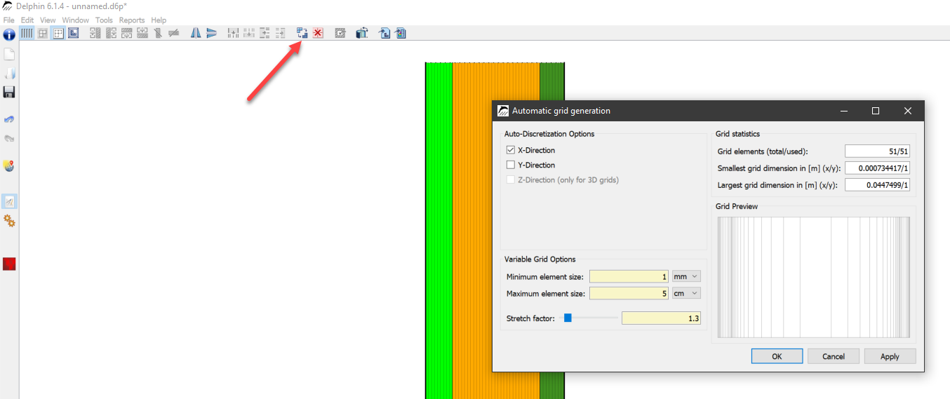
For this tutorial you don’t have to change the discretization. So you can close the dialog directly.
2.6. Initial and simulation conditions
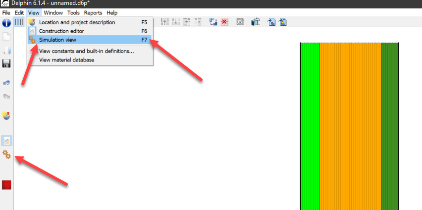
Now a look at the initial and simulation conditions. These have also already been defined by the project wizard. The dialog can be opened by a button (two gears), by Simulation View or by pressing F7.
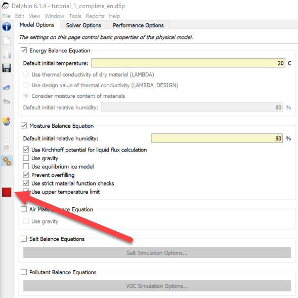
The dialog contains three tabs. In the first tab, basic settings for the physical models can be made. In this example the balance equations for energy and moisture are sufficient and should be activated.
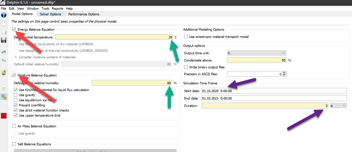
Important, further settings are the duration and the start time of the simulation. The project wizard has set 3 years as default. The global initial conditions concerning temperature and realtive humidity can be changed on the left side at the respective balance equations. A finer subdivision of the initial conditions is possible in another dialog. It is also useful to set the output time unit to days (d) or years (a), otherwise the x-axis unit of time is in hours, which is often too confusing. Now all project settings are complete and at the latest now the project should be saved (Ctrl+S).
2.7. Start simulation
In the same dialog on the right side the simulation can be started.
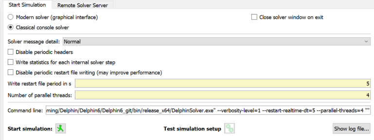
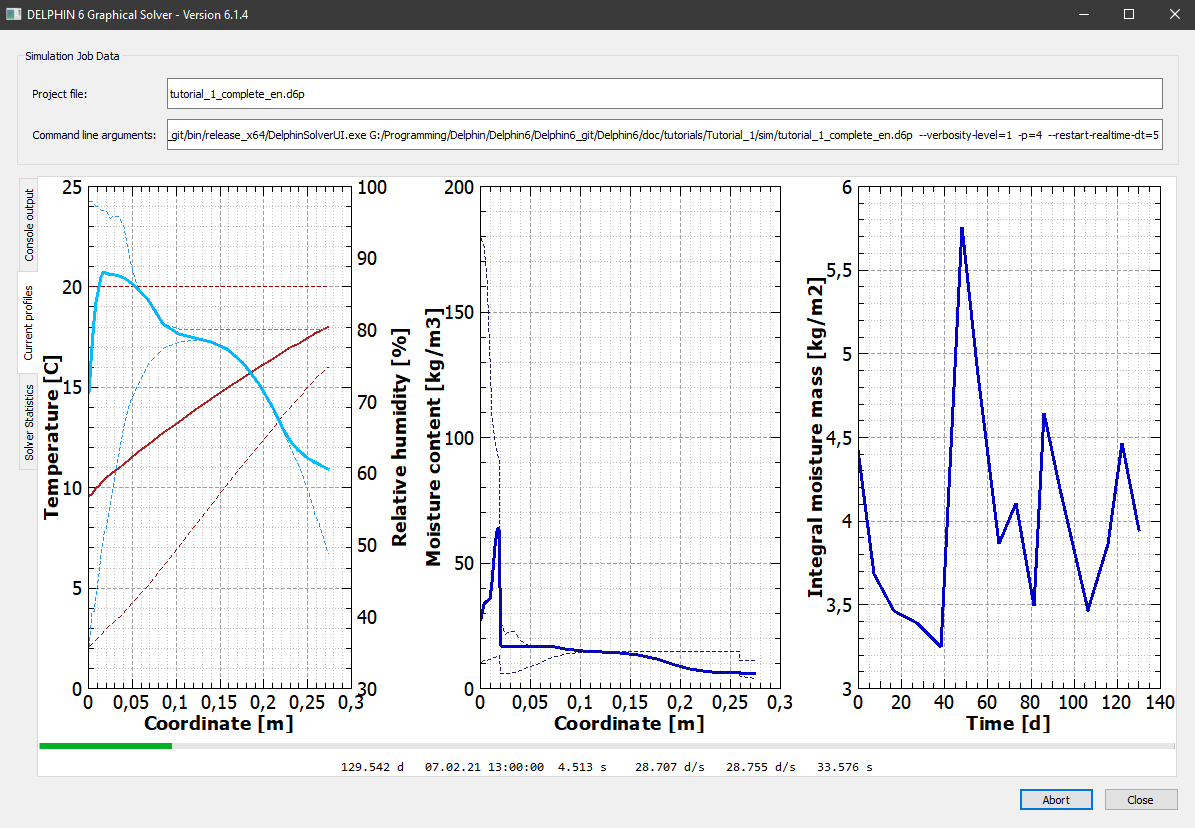
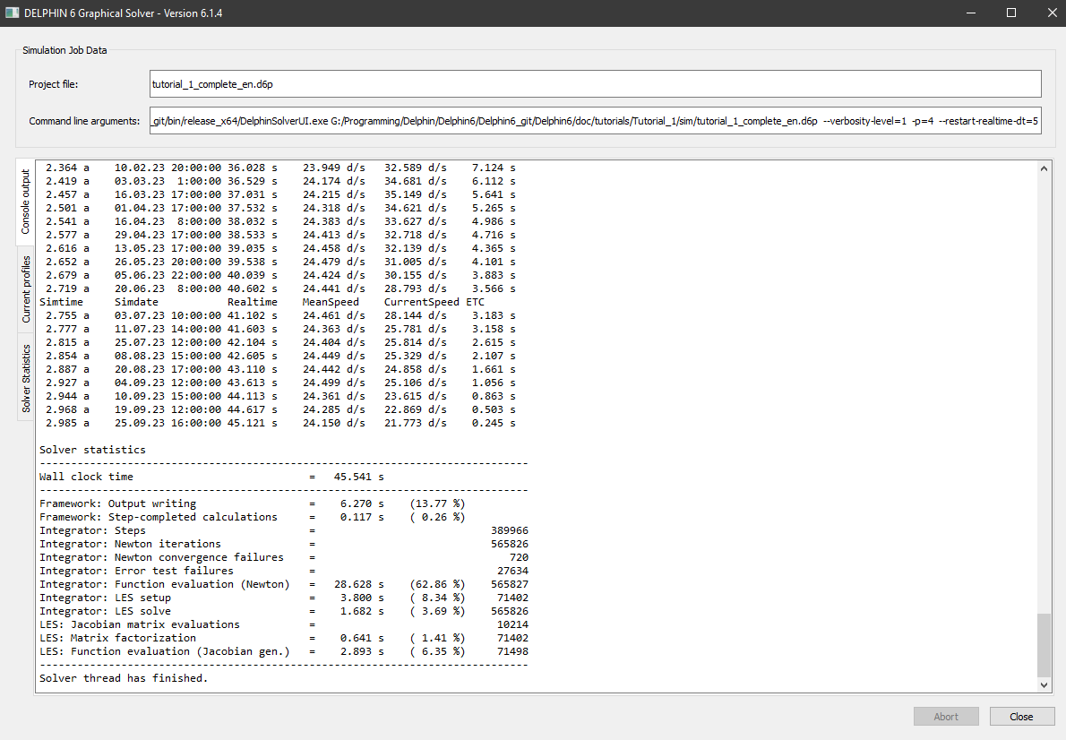
Here a solver can be selected. One that already shows graphical output during the simulation or an external solver. The latter is faster and generally recommended. In this example the solver with the graphical outputs is selected. In the dialog it is also possible to specify the number of parallel threads. Especially for 2D simulations, multiple threads can speed up a simulation many times. A click on 'Start simulation' starts the simulation and a window opens. The simulation window shows the current temperature, relative humidity and moisture profiles as well as the total moisture content over time, which is used to monitor the intermediate results of the simulation. Solver statistics and solver performance can also be viewed (left vertical tab 'Solver statistics').
The calculation results can be visualized already during the simulation with the post-processing program. The post-proc button starts the post-processor:
There are currently two different postprocessors: the old one from DELPHIN 5 and the newly developed version (PostProc2). The new postprocessing contains the most important features of the old version and should be used with priority. It also has new features which facilitate the evaluation and especially the comparison of data. For this tutorial PostProc 2 is used. PostProc 2 has to be installed before, because it is not included in the DELPHIN 6 setup. You will find the installer for it on the download page (http://www.bauklimatik-dresden.de/downloads.php) under PostProc. The default setting of the postprocessor can be changed in 'Edit >> Settings >> External programs'.
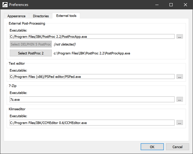
Click on the appropriate button of the postprocessor version to select it. After opening the PostProc 2 normally the data of the current project should already be loaded. If not, this data must be loaded from the project directory. For further information regarding the postprocessor: see tutorial 3 (for PostProc 2, PDF) on the website https://www.bauklimatik-dresden.de/delphin/2nd/doc/Tutorial_3_PP2_en.pdf. Furthermore there is an online help which you can reach under the following link: http://www.bauklimatik-dresden.de/postproc/help/en/index.html.
2.8. Reports
With version 6.1.4 an input report and with version 6.1.5 an output report has been added. Both reports and their settings can be found in the main menu under 'Reports'.
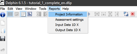
There are 4 submenu items here. The first two menu items are always available. The two reports are currently only available for 1D constructions, which are discretized in x-direction. This will be extended in future DELPHIN versions.
2.8.1. Project information
Clicking on this menu item opens a dialog where you can enter additional information about this project. This information will be used in the reports to make them more meaningful.
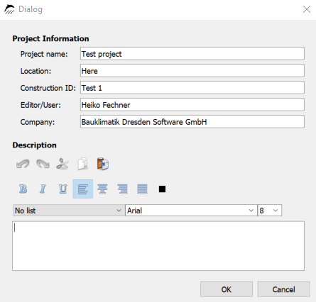
The information entered here will then appear at the top of all reports.
2.8.2. Assessment settings
In this dialog you can set which automatic assessments should be possible. Currently the following are available:
-
Check for long-term moistening - DIN 4108-3 D.7.2
-
Check for frost damage risk - DIN 4108-3 D.7.5
If these assessments are activated, the project must first be calculated afterwards so that the outputs generated by this are available to the assessment report.
2.8.3. Input data report
This report compiles the most important input data of the current project in a printable form. In version 6.1.5 this is only possible for 1D constructions in x-direction because other constructions cannot be displayed graphically yet. The following figure shows an example.
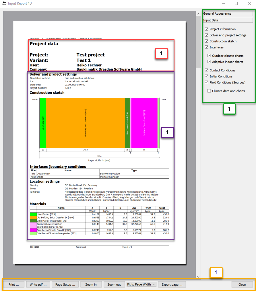
The following areas are highlighted:
-
Project information
-
Settings - which information should be displayed
-
Display of input data
-
Saving, printing and zooming
This report can be printed or saved as a pdf file. You can define in the settings what should be displayed.
2.8.4. Output report
The output report is used to display the assessments defined in the assessment settings. Furthermore, the project information and a selection of input data are displayed at the beginning. In version 6.1.5 there are two possible assessments.
Moisture accumulation
In DIN 4108-3 D.7.2 it is specified that the construction must be in a steady state for further evaluation. This also means that the total moisture mass must not continue to increase over the course of several years (moisture accumulation). This is checked in this section. First, it is checked whether the construction is already in a steady state for the selected calculation period. This is the case if the moisture content does not change by more than 1% from the end of one year to the end of the next. Such control also requires that the climate of one year has been applied cyclically. If this criterion is met, this assessment is completed positively. If there is still an increase, the calculation period can be further increased up to 10 years. If even then another moisture increase occurs, the evaluation is negative and the structure is not functional. Further evaluation is then no longer necessary. The report also shows the course of the moisture content in the entire construction.
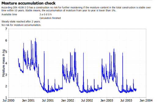
In our example, the moisture content actually decreases and the criterion is fulfilled.
Frost damage
DIN 4108-3 suggests in chapter D.7.5 a criterion to evaluate the risk of frost damage. This criterion checks whether the degree of saturation in an area of the construction exceeds 30% and at the same time the temperature falls below -5°C. If this evaluation is activated, DELPHIN generates an output for this criterion and evaluates it in this report.
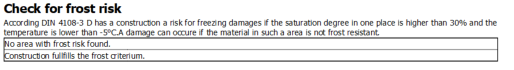
In our case, there is no risk. If areas for such a risk are found, a table with the areas and the materials in them is output here. The user must then check whether these materials are sensitive to frost.
3. Part 2 - Adding capillary conductive interior insulation
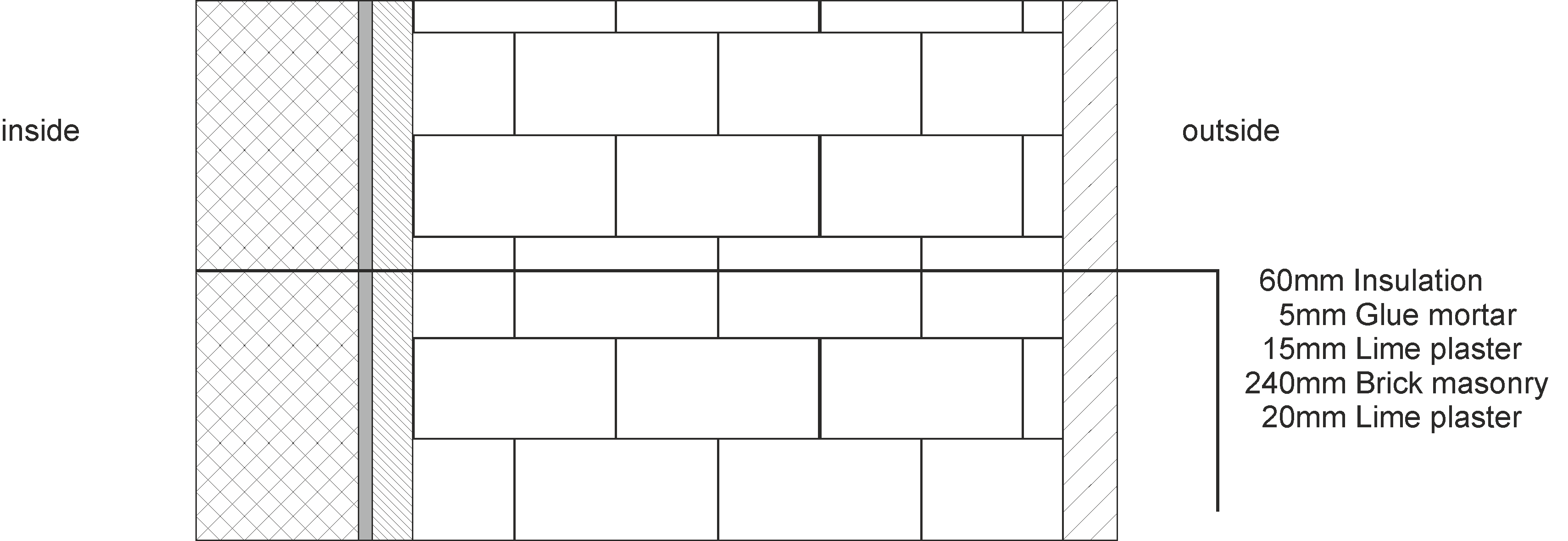
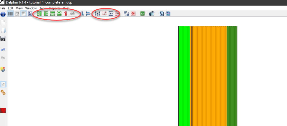
Since, among other things, the thermal resistance of the existing structure does not meet common modern requirements for comfort and energy savings, insulation is added. In this tutorial, it is assumed that it is not possible to add exterior insulation, e.g., because of a preserved façade, so a capillary highly conductive interior insulation made of calcium silicate (CaSi) is used. The CaSi insulation is applied with a system-compliant adhesive mortar. For comparison purposes, the project with the uninsulated existing structure should be preserved, so first the project should be saved under a different name, e.g. CaSi-80mm. Now the materials "Calsitherm KP Adhesive" (ID 705) and "Calsitherm Climatic Panel F" (ID 706) should be imported from the database into the project. Then two new layers can be added in the construction window on the left, inner layer with the corresponding thicknesses (8 mm adhesive mortar and 80 mm insulation). The buttons in the left ellipse (picture below) are available for this purpose.
Then the new layers can be added. To do this, select the innermost element and then click on the button for 'Add layer right'. Then the following dialog opens:
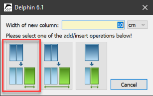
In the input line at the top you can specify the thickness of the new layer. Below there are three graphical buttons which show how to use this thickness:
-
Left - thickness corresponds to the entire new layer
-
Center - thickness corresponds to the construction width plus the new layer
-
Right - thickness corresponds to the selected column plus the new layer
If you simply want to add a new layer of the corresponding thickness, click the left button. Immediately after adding the new columns, the material of the layer that was last clicked is assigned to it. This assignment does not have to be removed now. It is enough to assign the previously added materials to the new layers. A material assigned later always overwrites the material assigned before. The assignment is done exactly as described in the chapter Outputs for the new output.
Finally, the automatic discretization dialog to the right of the right ellipse (picture above) can be called again or each new layer can be processed individually with the corresponding discretization dialog (buttons in the right ellipse).
Whenever the construction has been changed, it is advisable to check all boundary conditions and outputs to make sure they are still assigned to the correct layers. Surfaces/edges, on the other hand, are automatically assigned to the outer layers in 1D simulations. Here, all surface outputs except heat fluxes are incorrect. This can be easily seen by clicking, for example, on the 'Surface Temperature - Inner Surface' in the list. In the construction the assigned area is then marked dark.
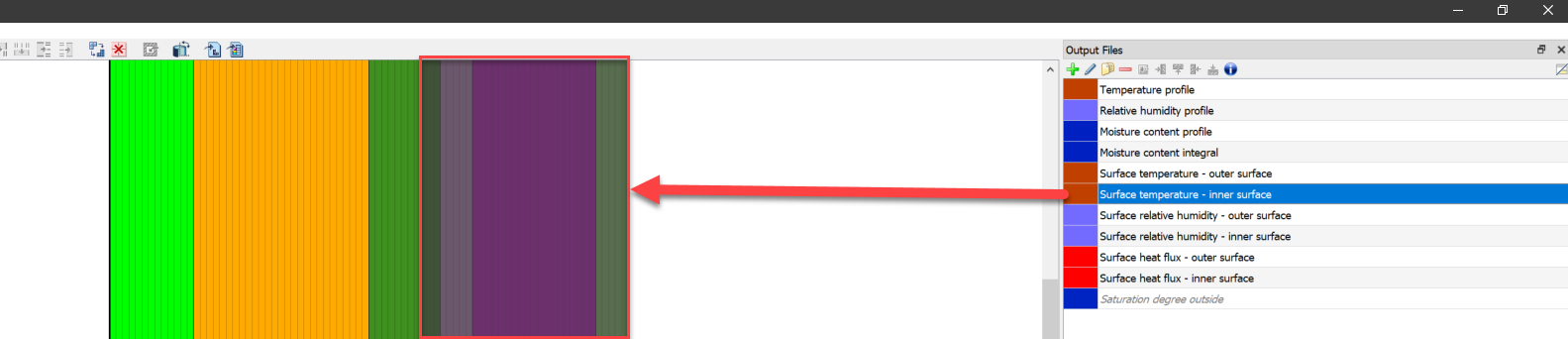
As you can see well in the image, now not only the surface is marked, but instead the old surface plus the new layers.
To set the output back to the new inner wall surface, the assignment must be changed. Assignment lists are normally hidden. They can be "dragged up", made visible by a button in the dialog window (red arrow) or all lists are accessed by 'Main Menu >> Window >> Allocation List Window Visible/Hidden'.
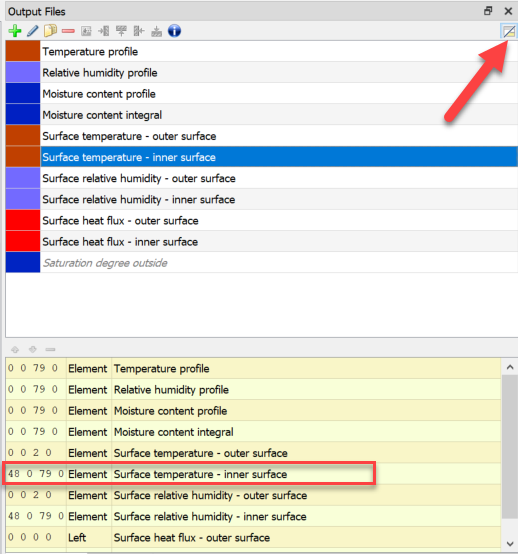
The assignment for the surface temperature is outlined in red in the image. The so-called element assignment is used here. The four numbers on the left mark the assigned area as element numbers. The numbers have the following meaning:
-
x1 y1 x2 y2
Since we have here a one-dimensional calculation in x-direction both y-coordinates are 0. X1 is 48 and x2 79. That means, here the output was assigned to all elements from number 48 to 79. Since we have 80 elements in total, element number 79 marks the rightmost one, i.e. the inner edge. These numbers can now be changed. Clicking in the number field opens the edit mode. Now you only have to change the 48 to 79 and again only the inner border element is marked. Analogously, one can adjust the other erroneous assignments.
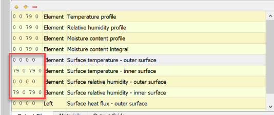
There is a second possibility for this. You can also delete the incorrect assignment in the assignment window (not the output in the output list). After that you just have to reassign the output.
Now the simulation can be run for the insulated construction.
4. Appendix A - Climate and boundary conditions
4.1. Create surfaces - boundary conditions
In the following, new surface (boundary) conditions are to be generated for the interior and exterior. In 1D calculation this is normally done by the project wizard. But sometimes you need other surfaces for variant analysis. Also, no standard surfaces are generated for 2D calculations.
A click on the green plus in the Surfaces/Borders dialog opens the corresponding dialog. In the context of this tutorial standard surfaces are used.
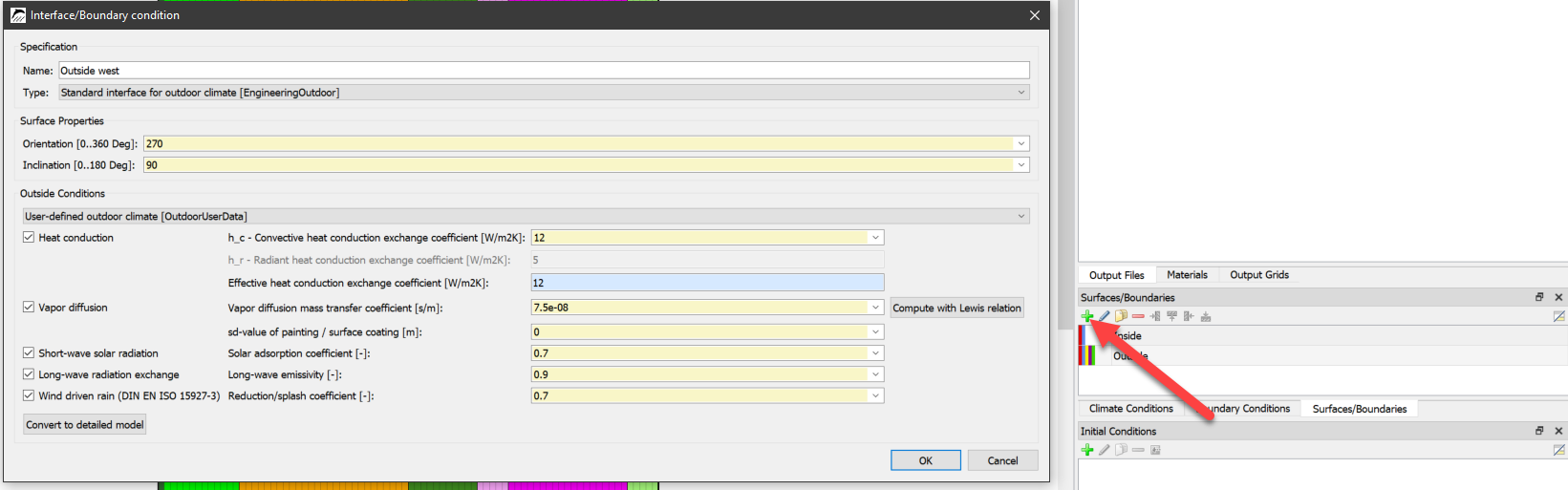
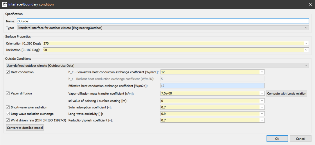
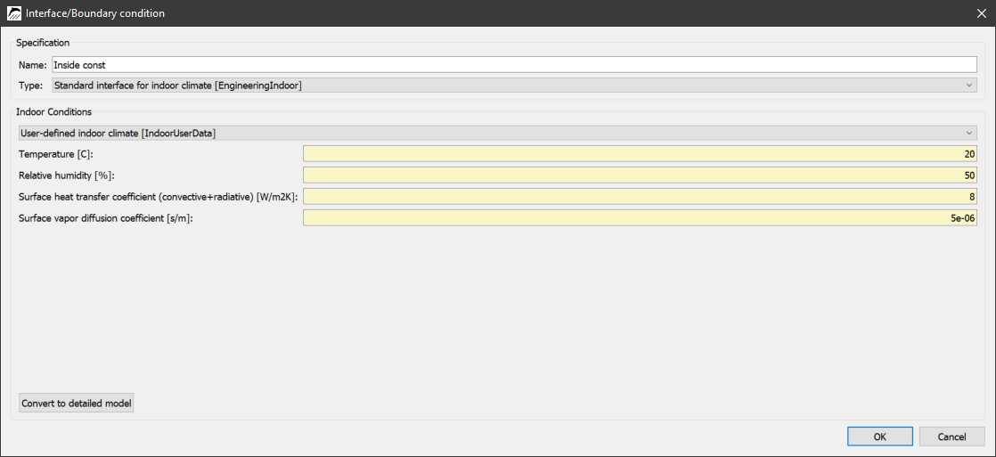
The left image shows the dialog for an exterior surface that faces west (270 degrees) and whose inclination is 90 degrees (vertical wall). The selected type "Standard outdoor climate" obtains the climate from the selected location or region (see project wizard). The outdoor climate condition should be set to "User defined …", then you can select exactly which climate components and parameters DELPHIN should calculate with. Afterwards, the indoor climate is generated, where the following settings have to be chosen:
After creating the surface conditions, they are assigned to the corresponding sides. This works analogously to the material assignment.
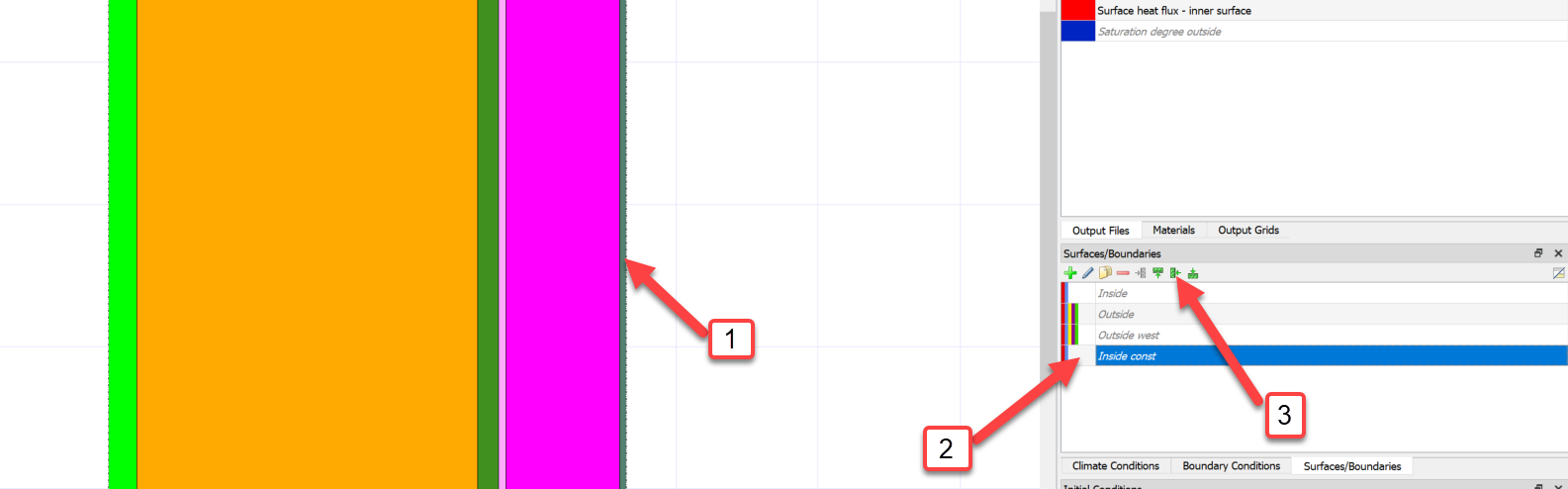
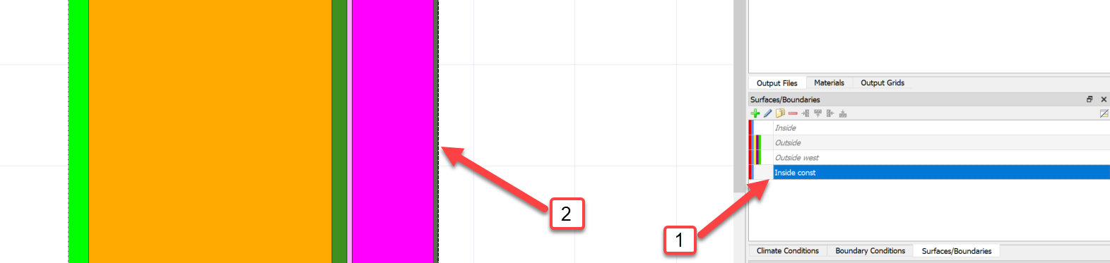
The interior climate is located on the right side. For the assignment a boundary layer has to be marked (1), the surface has to be marked (2) and at last it has to be assigned with a click for the assignment to a right side (3). (1) and (2) are also possible in reverse order. The external climate on the right side is assigned in the same way. For control, a surface condition can be clicked in the window Surfaces/Boundaries. Then the assigned surface will be highlighted by a dashed line.
In the procedure explained so far, only surfaces were created and assigned. These surfaces contain all necessary data to calculate boundary currents. We also call this methodology the simplified model. For more freedom in modeling and also more possibilities one can use the detailed model instead. Here, each surface acts as a container of boundary conditions, which must be created separately. The following graphic illustrates the relationships:
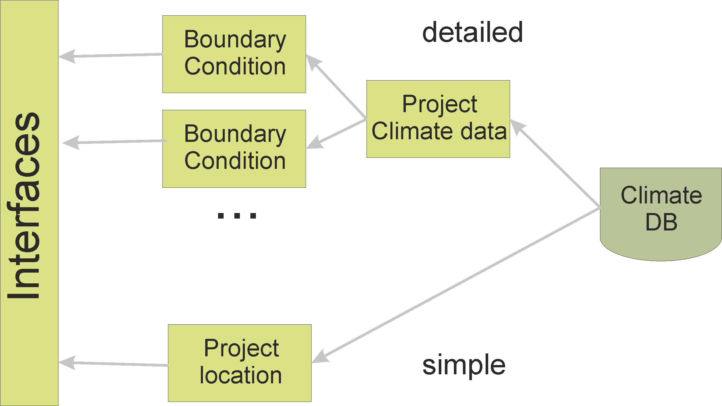
In the following, the handling of the detailed model will be explained in more detail. Here first climatic conditions and boundary conditions must be generated.
4.2. Generate climate conditions
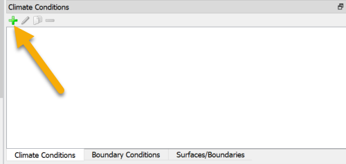
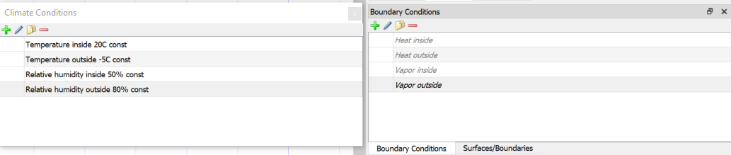
As mentioned before, the indoor and outdoor conditions or surfaces are not predefined, they are rather specified first by selecting and assigning climate and boundary conditions. This section shows how climate is defined manually. There are several ways to do this. For hygrothermal analyses, winter climate conditions are to be created. Specifically, this means an indoor temperature of 20°C with a relative humidity of 50%, and an outdoor temperature of -5°C and 80% humidity over a period of 90 days. The two climates are defined by a total of four climate conditions, which are generated first. For this, the window 'Climate conditions' must be called up first. As with all windows, a new definition is initiated by clicking the green '+' button.
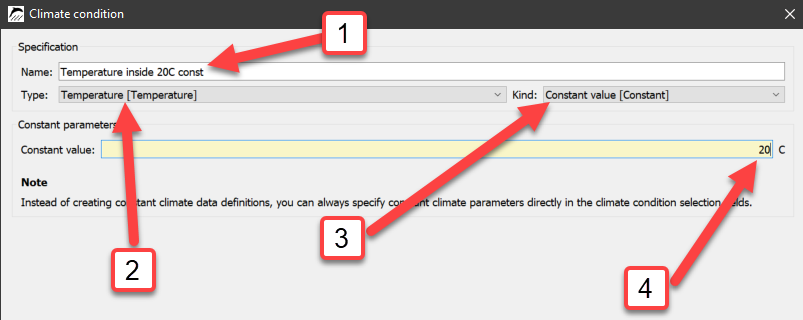
This will open a dialog for defining the climate condition. The following components are necessary: A name for identification (1), the temperature as the description of the climate type (2), the type of the course (3, here constant) and finally the value (4). If a climate data file is to be used, the path and the type of link are specified at this point.
The table below lists the names, type and values of the four conditions:
| Descriptive Name | Type | Kind | Value |
|---|---|---|---|
indoor temperature |
Temperature |
constant |
20 °C |
outdoor temperature |
Temperature |
constant |
-5 °C |
indoor relative humidity |
Relative Humidity |
constant |
50% |
outdoor relative humidity |
Relative Humidity |
constant |
80 % |
When all climate conditions are defined, the list looks like this:
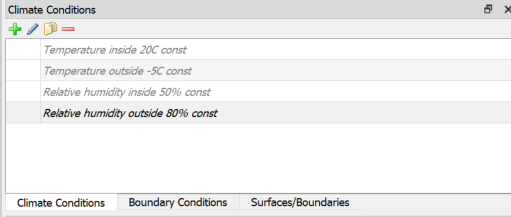
Here all definitions are shown in gray italics, because they are not used yet.
4.3. Generate boundary conditions
Climate data/conditions are necessary to be able to reference them in boundary conditions. Boundary conditions describe how the surface of the structure interacts with the climate and how it affects heat and moisture fluxes across the surfaces. Different physical effects such as heat conduction, vapor diffusion, air infiltration, water contact, etc. are each described in different boundary conditions. Analogous to the climate conditions, the window with the boundary conditions must be called up and four boundary conditions generated. After a click on the green '+' the first boundary condition can be defined.
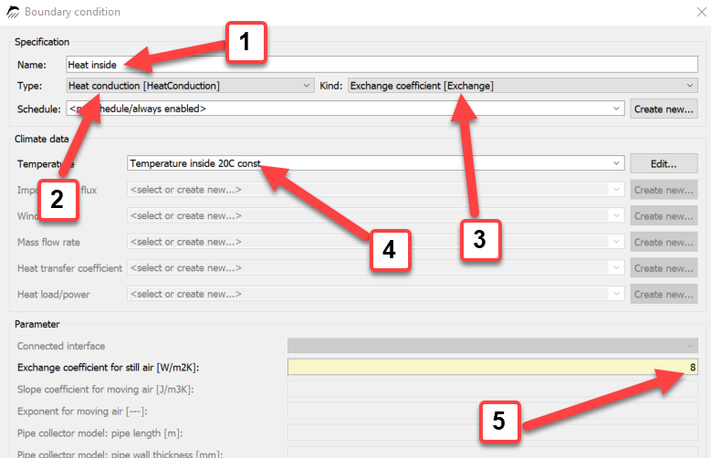
In the first field (1) a descriptive name should be chosen again. At (2) the type of boundary condition is determined (radiation, rain …) and at kind (3) the calculation model. At (4) the respective, already generated climate conditions have to be linked to this climate boundary condition, not needed climate conditions are grayed out. Finally, in the parameters section, the transition parameters are defined, e.g., for the heat conduction type, the relevant parameter is the heat transfer coefficient. Depending on the type of climatic boundary condition, it may be that no parameter is necessary. In this tutorial, longwave radiation is not modeled separately, so this is an effective heat transfer coefficient that includes a convective and longwave component (8 = 3 + 5 W/m2K). Within this example, the climate condition required is the indoor temperature generated in the last step.
The following table lists the names, types, nature and the parameters of the climate conditions for all four climate conditions. The parameters used correspond to the specifications of DIN 4108-3 D.2.3:
| Descriptive name | Type | Kind (model) | Parameters | Necessary climate condition |
|---|---|---|---|---|
Heat inside |
Heat conduction |
Exchange coefficient |
8 W/m2K |
Indoor temperature |
Heat outside |
heat conduction |
exchange coefficient |
17 W/m2K |
Outdoor temperature |
Vapor inside |
Vapor diffusion |
Exchange coefficient |
2.5e-8 s/m |
Indoor temperature Indoor humidity |
Vapor outside |
Vapor diffusion |
exchange coefficient |
7.5e-8 s/m |
Outdoor temperature Outdoor humidity |
The boundary conditions window should now contain all four boundary conditions as unused (italic gray) entries. The climate conditions, on the other hand, are now labeled as used (black).
4.4. Generate and assign surfaces (detailed).
Multiple boundary conditions can be combined into surfaces. Such surfaces or boundaries contain all boundary conditions on one surface.
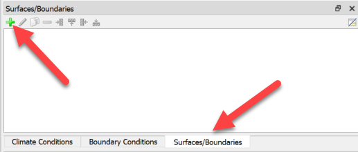
In the next step two surfaces/boundaries are generated, one for the inner and one for the outer surface. The green '+' in the surface/boundaries window calls a dialog for a new surface definition:
As with all other definitions in DELPHIN, a unique descriptive name should be assigned, e.g. 'indoor climate'. Within this example, the climate boundary conditions were created manually, so 'Detailed/scientific surface …' should be selected for Type. Then, depending on the surface, the corresponding climate boundary conditions should be selected, i.e. for the indoor surface 'Heat inside' and 'Vapor inside'.
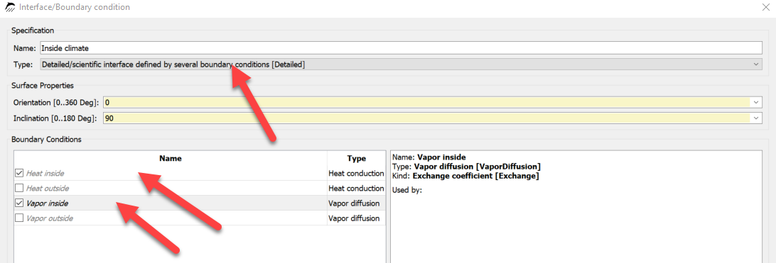
In the same way you can compose the surface for the "outdoor climate".
4.5. Further
To shorten the procedure described above there is another possibility to create detailed surfaces. One proceeds as follows:
-
Create simple surfaces
-
Convert these surfaces into detailed surfaces - click on 'Convert to detailed model'.
-
all corresponding climate and boundary conditions will be created automatically
-
-
Adjustment of climate and boundary conditions
This methodology is faster but has a higher risk of incorrect input.
5. Appendix B - Outputs
5.1. Time grid for outputs
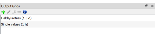
Before the actual output variables are defined and assigned, the time grids for the outputs should be defined. This is done in the Output Grid window. It is very useful to limit the output of fields ("colored images"). Therefore (at least) two grids should be defined, one for fields and profiles, and one for scalars (single values), where for larger areas (amount of water in several layers) or single points (humidity in the edge of a room) only one output value per time unit should be output.
With the '+' button a new output schedule is generated in the output schedule window, which should be given a unique name (1). The output frequency does not have to remain constant during the simulation, but can be varied by setting intervals (2).
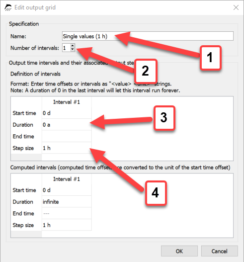
For each interval, the duration of the interval (3) and the output time grid during the interval (4) must be determined. Alternatively, the start or end time of the interval can be specified, where time in this case means the relative time since the start of the simulation. If an interval duration of 0 d (a time unit must not be forgotten here either) is specified for the last (or the only) interval, it means that this element will remain until the end of the simulation, no matter how long it will last. For this tutorial, two intervals are to be created, one with an output interval of 12 h, e.g. named "Profile (12h)", and one with an output interval of 1 h for scalars.
5.2. Output files
Now the outputs themselves can be defined. This is done by generating output files. In the window for output files, a new output should now be generated with the '+' button, as always by setting a suitable identification name (1). It should be noted that the later output file will be named after this name. Therefore, do not use characters that are not allowed for file names, e.g. slashes or semi-colons.
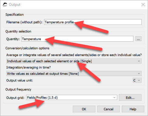
Next, the physical quantity of the output is selected, e.g. temperature or relative humidity (2). In the selection list that opens (after a click on ), all output types are included that can be calculated with DELPHIN.
Now the type "temperature" can be selected from the list.
To quickly navigate through the table, simply click on a cell in the Name or Description column and type the first letter of the name or description. The cursor will then jump to the corresponding cells. It is also possible to arrange the table by type or name (alphabetically). Furthermore, all more frequently used sizes are displayed in bold at the top (can be switched off with a check mark at the bottom left).
The selected type also determines the default output unit and whether the output can be assigned to elements or element boundaries. Finally, the output time grid is selected, which defines in which time intervals an output value is written.
Now the window of output files should contain a single output "temperature profile". During discretization the whole construction was discretized into single elements. This output can now be assigned to the entire construction, which means that at each output time a value is stored for each individual element, so that ultimately temperature profiles will be created through the entire wall construction (see Post-Processing in Part 2 of this tutorial).
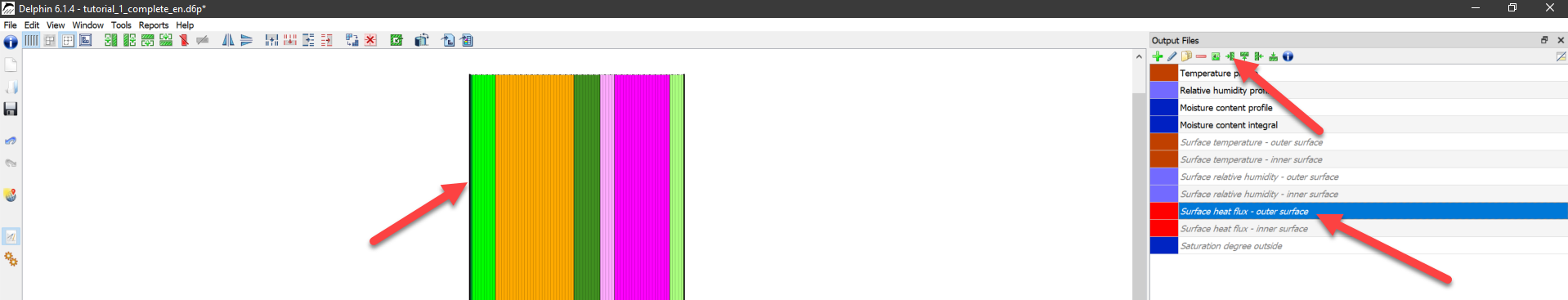
All elements of a construction can be selected by mouse click and pressing the Shift key or by pressing Ctrl+a. Then the corresponding output file can be selected and then assigned with the button. Also in this window the letters of the output definition will change from gray-italic to black-straight indicating that the output is used.
It is also possible to calculate the average from the results of many elements. For example, the weighted average value ("[Mean]") or the sum of the result values of the elements ("[Integral]") can be calculated, for example the integral amount of water of the whole construction. These space-related operations in result calculation are called Space Type (3) of the output and can be determined in the output definition dialog. If an output is to record the result value of each individual element (default), the Space Type is " … [Single]".
Simulation outputs are time-dependent quantities, so there are some time-related output options, called Time Type, in DELPHIN. For example, it is possible to average in time (at Time Integration/Averaging " … [Mean]"). This time averaging starts with the start of the simulation. Flows or sources can also be integrated in time with the setting " … [Integral]". If the value is to be stored exactly at the output time, the type "[None]" is to be selected. All these parameters are set in the dialog of the respective output.
The following outputs, among others, can be useful in many simulations:
| Output name | Quantity | Time grid | Space type | Time type |
|---|---|---|---|---|
Profile - Temperature |
Temperature |
Fields/Profiles (1.5 d) |
Single |
None |
Profile - Relative Humidity |
RelativeHumidity |
Fields/Profile (1.5 d) |
Single |
None |
Profile - Water Content |
MoistureMassDensity |
Fields/Profile (1.5 d) |
Single |
None |
Total - Moisture |
MoistureMassDensity |
Single (1 h) |
Integral |
None |
Total - Liquid Water |
OverhygroscopicWaterMassDensity |
Single Values (1 h) |
Integral |
None |
Temperature Surface Inside |
Temperature |
Single Values (1 h) |
Mean |
None |
Relative Humidity Indoor Surface |
RelativeHumidity |
Single Values (1 h) |
Mean |
None |
Degree of Saturation outside medium |
DegreeOfSaturation |
Single Values (1 h) |
Mean |
None |
Temperature outside medium |
Temperature |
Single values (1 h) |
Mean |
None |
Surface Heat Flux - Outside Surface |
TotalHeatFlux |
Individual Values (1 h) |
Mean |
None |
Surface Heat Flux - Inner Surface |
TotalHeatFlux |
Individual Values (1 h) |
Mean |
Mean |
For all outputs, except the heat fluxes, the instantaneous values (NONE) are set for the time response. The output value therefore corresponds to the value that was valid exactly at the output time. For the heat flows, a time average value (MEAN) was selected instead. Here the output value corresponds to the average value from the last output time to the current one. For the calculation of average heat losses one can select here also INTEGRAL. Then all heat losses are added up over the time. To calculate a mean value you only have to take the first and the last value of a time interval, calculate the difference and divide the result by the length of the time interval.
If several output conditions of one type or similar type are to be used, they do not have to be redefined each time. Outputs can simply be copied.
All output data except the last one can be assigned to the whole construction. The flux output is used to obtain the total heat flux in the construction, which changes dynamically depending on the fluxes entering and leaving the construction.
Outputs from flows/fluxes are often assigned to surfaces/boundaries. In this tutorial, it should be assigned to the first element on the left (outer surface) and to the last element on the right (inner surface). First, only the first, left element is to be selected and then the output "Surface heat flux - outer surface" is to be assigned to it using the "Assign from left" button. Afterwards, this output can also be assigned to the last, right element. If now this output is clicked, both sides will be highlighted.
Due to the small thickness of the discretized elements near layer boundaries, the assignment at these locations is difficult (except with very high zoom). Alternatively, all elements of the construction can be displayed on the screen in the same thickness (equidistant). You can switch between proportional and equidistant display with the button (top left of the construction window).
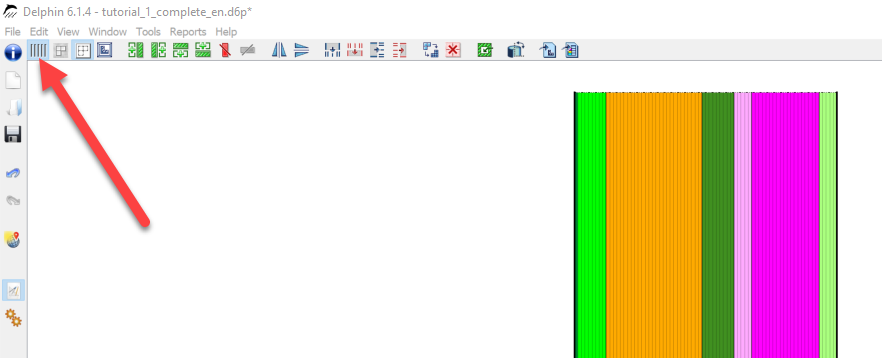 Image 60. Button for equidistant view
After all output definitions are set, the project is ready for simulation.